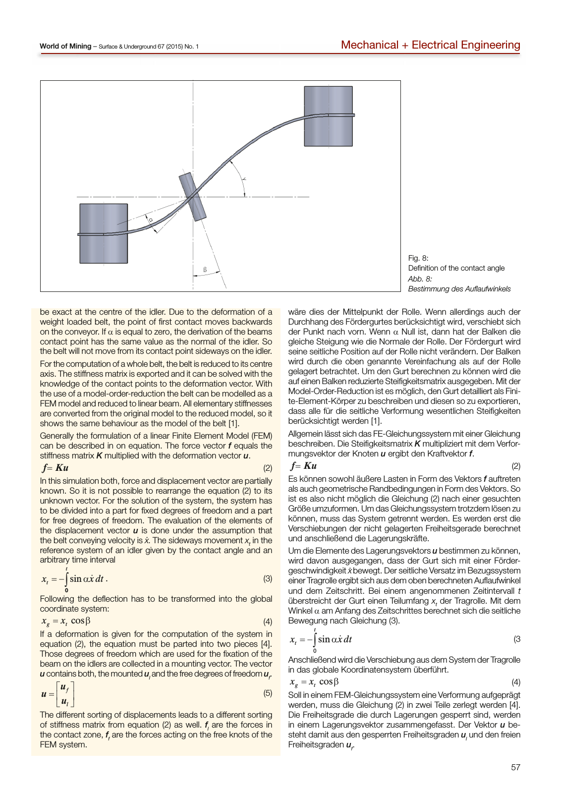
57 World of Mining Surface Underground 67 2015 No 1 Mechanical Electrical Engineering be exact at the centre of the idler Due to the deformation of a weight loaded belt the point of first contact moves backwards on the conveyor If α is equal to zero the derivation of the beams contact point has the same value as the normal of the idler So the belt will not move from its contact point sideways on the idler For the computation of a whole belt the belt is reduced to its centre axis The stiffness matrix is exported and it can be solved with the knowledge of the contact points to the deformation vector With the use of a model order reduction the belt can be modelled as a FEM model and reduced to linear beam All elementary stiffnesses are converted from the original model to the reduced model so it shows the same behaviour as the model of the belt 1 Generally the formulation of a linear Finite Element Model FEM can be described in on equation The force vector f equals the stiffness matrix K multiplied with the deformation vector u f Ku 2 In this simulation both force and displacement vector are partially known So it is not possible to rearrange the equation 2 to its unknown vector For the solution of the system the system has to be divided into a part for fixed degrees of freedom and a part for free degrees of freedom The evaluation of the elements of the displacement vector u is done under the assumption that the belt conveying velocity is x The sideways movement xt in the reference system of an idler given by the contact angle and an arbitrary time interval sin t tx xdt α 0 3 Following the deflection has to be transformed into the global coordinate system cosg tx x β 4 If a deformation is given for the computation of the system in equation 2 the equation must be parted into two pieces 4 Those degrees of freedom which are used for the fixation of the beam on the idlers are collected in a mounting vector The vector u contains both the mounted ul and the free degrees of freedom uf f l u u u 5 The different sorting of displacements leads to a different sorting of stiffness matrix from equation 2 as well fl are the forces in the contact zone ff are the forces acting on the free knots of the FEM system wäre dies der Mittelpunkt der Rolle Wenn allerdings auch der Durchhang des Fördergurtes berücksichtigt wird verschiebt sich der Punkt nach vorn Wenn α Null ist dann hat der Balken die gleiche Steigung wie die Normale der Rolle Der Fördergurt wird seine seitliche Position auf der Rolle nicht verändern Der Balken wird durch die oben genannte Vereinfachung als auf der Rolle gelagert betrachtet Um den Gurt berechnen zu können wird die auf einen Balken reduzierte Steifigkeitsmatrix ausgegeben Mit der Model Order Reduction ist es möglich den Gurt detailliert als Fini te Element Körper zu beschreiben und diesen so zu exportieren dass alle für die seitliche Verformung wesentlichen Steifigkeiten berücksichtigt werden 1 Allgemein lässt sich das FE Gleichungssystem mit einer Gleichung beschreiben Die Steifigkeitsmatrix K multipliziert mit dem Verfor mungsvektor der Knoten u ergibt den Kraftvektor f f Ku 2 Es können sowohl äußere Lasten in Form des Vektors f auftreten als auch geometrische Randbedingungen in Form des Vektors So ist es also nicht möglich die Gleichung 2 nach einer gesuchten Größe umzuformen Um das Gleichungssystem trotzdem lösen zu können muss das System getrennt werden Es werden erst die Verschiebungen der nicht gelagerten Freiheitsgerade berechnet und anschließend die Lagerungskräfte Um die Elemente des Lagerungsvektors u bestimmen zu können wird davon ausgegangen dass der Gurt sich mit einer Förder geschwindigkeit x bewegt Der seitliche Versatz im Bezugssystem einer Tragrolle ergibt sich aus dem oben berechneten Auflaufwinkel und dem Zeitschritt Bei einem angenommenen Zeitintervall t überstreicht der Gurt einen Teilumfang xt der Tragrolle Mit dem Winkel α am Anfang des Zeitschrittes berechnet sich die seitliche Bewegung nach Gleichung 3 sin t tx xdt α 0 3 Anschließend wird die Verschiebung aus dem System der Tragrolle in das globale Koordinatensystem überführt cosg tx x β 4 Soll in einem FEM Gleichungssystem eine Verformung aufgeprägt werden muss die Gleichung 2 in zwei Teile zerlegt werden 4 Die Freiheitsgrade die durch Lagerungen gesperrt sind werden in einem Lagerungsvektor zusammengefasst Der Vektor u be steht damit aus den gesperrten Freiheitsgraden ul und den freien Freiheitsgraden uf Fig 8 Definition of the contact angle Abb 8 Bestimmung des Auflaufwinkels

Hinweis: Dies ist eine maschinenlesbare No-Flash Ansicht.
Klicken Sie hier um zur Online-Version zu gelangen.